ai学习：现代卷积神经网络

LeNet

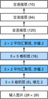
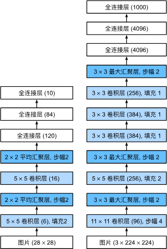
LeNet 的总体架构如下：

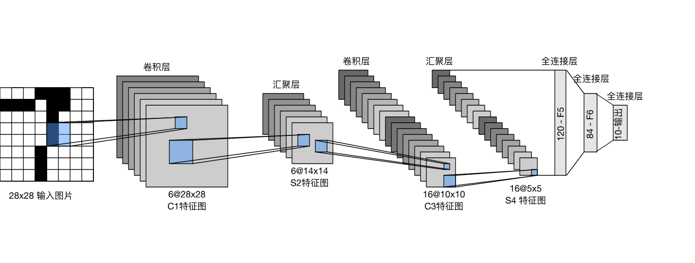
LeNet-5 由两个特征提取器和三个分类器组成：

• 每个特征提取器包含一个用于提取输入图像的局部特征的卷积层 (Convolutional Layers) 和一个用于下采样、提高变形鲁棒性的平均池化层 (Average Pooling Layers)；
• 每个分类器都是一个全连接层 (Fully Connected Layers)，用于整合特征提取器生成的高维特征，并降维映射到具体的输出类别。
• 在这个过程中，每经过一次卷积层，特征图的高度和宽度都减小，而通道不断增加。池化层在保持通道不变的情况下进一步减半特征图的尺寸。最后，将特征降维展平后，使用全连接层输出各个结果的概率。

‍

模型定义

模型定义如下：

#导入所需的库
import torch
from torch import nn
from d2l import torch as d2l
#定义网络结构
net = nn.Sequential(
    nn.Conv2d(1, 6, kernel_size=5, padding=2), nn.Sigmoid(),
    nn.AvgPool2d(kernel_size=2, stride=2),
    nn.Conv2d(6, 16, kernel_size=5), nn.Sigmoid(),
    nn.AvgPool2d(kernel_size=2, stride=2),

    # 分类器（展平后依次进入三个全连接层）
    nn.Flatten(),
    nn.Linear(16 * 5 * 5, 120), nn.Sigmoid(),
    nn.Linear(120, 84), nn.Sigmoid(),
    nn.Linear(84, 10))

为了方便看每个层的样子，可以打印出来

#把每一层数据的shape给打印出来
X = torch.rand(size=(1, 1, 28, 28), dtype=torch.float32)#创建符合要求的张量
for layer in net:
    X = layer(X)#通过每一层
    print(layer.__class__.__name__,'output shape: \t',X.shape)#打印

Conv2d output shape: 	 torch.Size([1, 6, 28, 28])
Sigmoid output shape: 	 torch.Size([1, 6, 28, 28])
AvgPool2d output shape: 	 torch.Size([1, 6, 14, 14])
Conv2d output shape: 	 torch.Size([1, 16, 10, 10])
Sigmoid output shape: 	 torch.Size([1, 16, 10, 10])
AvgPool2d output shape: 	 torch.Size([1, 16, 5, 5])
Flatten output shape: 	 torch.Size([1, 400])
Linear output shape: 	 torch.Size([1, 120])
Sigmoid output shape: 	 torch.Size([1, 120])
Linear output shape: 	 torch.Size([1, 84])
Sigmoid output shape: 	 torch.Size([1, 84])
Linear output shape: 	 torch.Size([1, 10])

模型训练

现在我们已经实现了 LeNet，接下来看看 LeNet 在 Fashion-MNIST 数据集上的表现。

batch_size = 256#批量大小
train_iter, test_iter = d2l.load_data_fashion_mnist(batch_size=batch_size)#下载或加载数据集，得到训练和测试集的迭代对象

测试函数和训练函数如下：

由于完整的数据集位于内存中，因此在模型使用 GPU 计算数据集之前，我们需要将其复制到显存中。

def evaluate_accuracy_gpu(net, data_iter, device=None): #@save
    """使用GPU计算模型在数据集上的精度"""
    if isinstance(net, nn.Module):
        net.eval()  # 设置为评估模式
        if not device:
            device = next(iter(net.parameters())).device
    # 正确预测的数量，总预测的数量
    metric = d2l.Accumulator(2)#创建一个累加器，包含2个要累加的元素
    with torch.no_grad():
        for X, y in data_iter:
            if isinstance(X, list):
                # BERT微调所需的（之后将介绍）
                X = [x.to(device) for x in X]
            else:
                X = X.to(device)
            y = y.to(device)
            metric.add(d2l.accuracy(net(X), y), y.numel())#把每一组数据预测结果正确的个数和长度累加
    return metric[0] / metric[1]

#@save
def train_ch6(net, train_iter, test_iter, num_epochs, lr, device):
    """用GPU训练模型(在第六章定义)"""
    def init_weights(m):
        if type(m) == nn.Linear or type(m) == nn.Conv2d:
            nn.init.xavier_uniform_(m.weight)#对linear类型的层用xavier初始化
    net.apply(init_weights)
    print('training on', device)
    net.to(device)
    optimizer = torch.optim.SGD(net.parameters(), lr=lr)
    loss = nn.CrossEntropyLoss()
    animator = d2l.Animator(xlabel='epoch', xlim=[1, num_epochs],
                            legend=['train loss', 'train acc', 'test acc'])#动画需要
    timer, num_batches = d2l.Timer(), len(train_iter)
    for epoch in range(num_epochs):
        # 训练损失之和，训练准确率之和，范例数
        metric = d2l.Accumulator(3)
        net.train()
        for i, (X, y) in enumerate(train_iter):
            timer.start()
            optimizer.zero_grad()#梯度清零
            X, y = X.to(device), y.to(device)
            y_hat = net(X)#正向传播
            l = loss(y_hat, y)#计算损失
            l.backward()#反向传播
            optimizer.step()#梯度下降
            with torch.no_grad():
                metric.add(l * X.shape[0], d2l.accuracy(y_hat, y), X.shape[0])#训练损失之和，训练准确率之和，范例数
            timer.stop()
            train_l = metric[0] / metric[2]
            train_acc = metric[1] / metric[2]
            if (i + 1) % (num_batches // 5) == 0 or i == num_batches - 1:
                animator.add(epoch + (i + 1) / num_batches,
                             (train_l, train_acc, None))
        test_acc = evaluate_accuracy_gpu(net, test_iter)#评估测试集的精度
        animator.add(epoch + 1, (None, None, test_acc))
    print(f'loss {train_l:.3f}, train acc {train_acc:.3f}, '
          f'test acc {test_acc:.3f}')
    print(f'{metric[2] * num_epochs / timer.sum():.1f} examples/sec '
          f'on {str(device)}')

lr, num_epochs = 0.9, 10
train_ch6(net, train_iter, test_iter, num_epochs, lr, d2l.try_gpu())

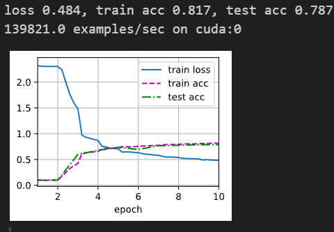
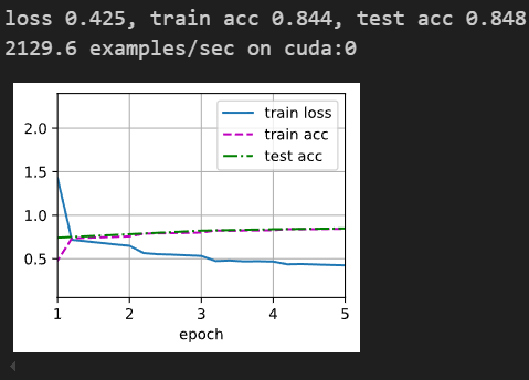
最终结果：

AlexNet

在 2012 年前，图像特征都是机械地计算出来的。事实上，设计一套新的特征函数、改进结果，并撰写论文是盛极一时的潮流。

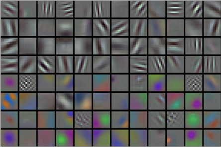
但是深度学习领域的观点认为，深度学习模型应该能自动学习到数据的特征，而不依赖于传统机器学习中的手工特征提取。这些特征由多个神经网络层共同学习到。靠近输入层的特征表示通常用于检测图像的低级特征（边缘、颜色和纹理等）；位于网络更深层次、靠近输出层的特征表示，由多个低级特征抽象而来，用于表示形状结构、物体部件和语义信息等。最终，通过隐藏的神经元表示图像的综合信息，实现分类与判别。

2012 提出的 AlexNet 使用 8 层卷积神经网络以巨大优势赢得了当年的 ImageNet 图像识别挑战赛，首次证明了模型能自动学习特征的能力，改变了计算机视觉研究的格局。

在 AlexNet 网络的最底层，模型学习到了一些类似于传统滤波器的特征抽取器，下图是提取出来的图像特征：

AlexNet 和 LeNet 的架构非常相似，但也有许多的不同：

• AlexNet 具有比 LeNet5 ​更深的网络结构、更大的通道数：AlexNet 由 5 个卷积层、2 个全连接隐藏层和 1 个全连接输出层组成。ImageNet 的图像像素分辨率是 Fashion-MNIST 数据集的 10 倍多，需要更大的 (11×11) 卷积窗口捕获目标；
• AlexNet 连接最后一个卷积层的全连接层共有 4096 个输出：当时由于 GPU 显存的限制，需要​采用双数据流的方式，每个 GPU 只能计算一半的参数。现在的 GPU 显存充裕，很少需要跨 GPU 分解模型，可对其进行精简。
• AlexNet 的每个卷积层和全连接层​使用非饱和激活函数 ReLU：而不用容易导致梯度消失/爆炸的 Sigmoid 函数激活。一方面，ReLU 函数的计算更简单，不需要复杂的求幂运算；另一方面，ReLU 激活函数在正区间的梯度总是 1，使模型即使没有很好地初始化，也能有效地完成训练，而不会导致梯度消失/爆炸的问题；
• AlexNet 在权重衰减的基础上使用暂退技术控制全连接层的模型复杂度；
• AlexNet 通过翻转、裁切和变色对数据集进行了图像的​数据增强，更大的样本量进一步减少了过拟合的问题。

模型定义代码如下：

import torch
from torch import nn
from d2l import torch as d2l

net = nn.Sequential(
    # 这里，我们使用一个11*11的更大窗口来捕捉对象。
    # 同时，步幅为4，以减少输出的高度和宽度。
    # 另外，输出通道的数目远大于LeNet
    nn.Conv2d(1, 96, kernel_size=11, stride=4, padding=1), nn.ReLU(),
    nn.MaxPool2d(kernel_size=3, stride=2),
    # 减小卷积窗口，使用填充为2来使得输入与输出的高和宽一致，且增大输出通道数
    nn.Conv2d(96, 256, kernel_size=5, padding=2), nn.ReLU(),
    nn.MaxPool2d(kernel_size=3, stride=2),
    # 使用三个连续的卷积层和较小的卷积窗口。
    # 除了最后的卷积层，输出通道的数量进一步增加。
    # 在前两个卷积层之后，汇聚层不用于减少输入的高度和宽度
    nn.Conv2d(256, 384, kernel_size=3, padding=1), nn.ReLU(),
    nn.Conv2d(384, 384, kernel_size=3, padding=1), nn.ReLU(),
    nn.Conv2d(384, 256, kernel_size=3, padding=1), nn.ReLU(),
    nn.MaxPool2d(kernel_size=3, stride=2),
    nn.Flatten(),
    # 这里，全连接层的输出数量是LeNet中的好几倍。使用dropout层来减轻过拟合
    nn.Linear(6400, 4096), nn.ReLU(),
    nn.Dropout(p=0.5),
    nn.Linear(4096, 4096), nn.ReLU(),
    nn.Dropout(p=0.5),
    # 最后是输出层。由于这里使用Fashion-MNIST，所以用类别数为10，而非论文中的1000
    nn.Linear(4096, 10))

X = torch.randn(1, 1, 224, 224)
for layer in net:
    X=layer(X)
    print(layer.__class__.__name__,'output shape:\t',X.shape)

Conv2d output shape:	 torch.Size([1, 96, 54, 54])
ReLU output shape:	 torch.Size([1, 96, 54, 54])
MaxPool2d output shape:	 torch.Size([1, 96, 26, 26])
Conv2d output shape:	 torch.Size([1, 256, 26, 26])
ReLU output shape:	 torch.Size([1, 256, 26, 26])
MaxPool2d output shape:	 torch.Size([1, 256, 12, 12])
Conv2d output shape:	 torch.Size([1, 384, 12, 12])
ReLU output shape:	 torch.Size([1, 384, 12, 12])
Conv2d output shape:	 torch.Size([1, 384, 12, 12])
ReLU output shape:	 torch.Size([1, 384, 12, 12])
Conv2d output shape:	 torch.Size([1, 256, 12, 12])
ReLU output shape:	 torch.Size([1, 256, 12, 12])
MaxPool2d output shape:	 torch.Size([1, 256, 5, 5])
Flatten output shape:	 torch.Size([1, 6400])
Linear output shape:	 torch.Size([1, 4096])
ReLU output shape:	 torch.Size([1, 4096])
Dropout output shape:	 torch.Size([1, 4096])
Linear output shape:	 torch.Size([1, 4096])
ReLU output shape:	 torch.Size([1, 4096])
Dropout output shape:	 torch.Size([1, 4096])
Linear output shape:	 torch.Size([1, 10])

训练与测试如下：

batch_size = 128
train_iter, test_iter = d2l.load_data_fashion_mnist(batch_size, resize=224)
lr, num_epochs = 0.01, 5
d2l.train_ch6(net, train_iter, test_iter, num_epochs, lr, d2l.try_gpu())

VGG

之前的 AlexNet 证明了模型能自动学习特征的能力，但这一突破并没有为后续的研究提供用于构建新网络的模板。但 AlexNet 的积极意义之一是意识到了卷积神经网络的基本结构由带填充以保持分辨率的卷积层、ReLU 等非线性激活函数，以及池化层组成。随着深度学习网络设计模式的发展，这种网络基本结构能在更大的尺度上复用，而使研究者的视角从“神经元”到“层”，又逐步转向“块”。

与 AlexNet、LeNet 一样，VGG 网络可以分为两部分：第一部分主要由卷积层和汇聚层组成，第二部分由全连接层组成。

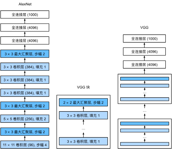
我们先来实现一个 VGG 块，VGG 块的其中一种形式是：由两层使用 ReLU 激活函数的 3×3 填充为 1 的卷积层，后接一个 2×2 步幅为 2 的最大池化层组成。可以在卷积时保持宽高、在池化时宽高分辨率减半。

#VGG块
def vgg_block(num_convs, in_channels, out_channels):#块中卷积层数，输入输出通道数
    layers = []
    for _ in range(num_convs):#用for循环
        layers.append(nn.Conv2d(
            in_channels, out_channels, kernel_size=3, padding=1))
        layers.append(nn.ReLU())
        in_channels = out_channels#添加一层后取当前输出通道数为下一层输入通道数，
        #这里说明VGG块改变通道数的方法是在第一层就将通道数改变好，后面层中通道数全不变
    layers.append(nn.MaxPool2d(kernel_size=2, stride=2))
    return nn.Sequential(*layers)

VGG 网络同样由卷积层、汇聚层组成的特征提取模块和由全连接层组成的分类模块组成。原始 VGG 网络有 5 个卷积块，其中前两个块各有一个卷积层，后三个块各包含两个卷积层。 第一个模块有 64 个输出通道，每个后续模块将输出通道数量翻倍，直到该数字达到 512。由于该网络使用 8 个卷积层和 3 个全连接层，因此它通常被称为 VGG-11。实现如下：

#每个VGG块的（卷积层数，输出通道数）
conv_arch = ((1, 64), (1, 128), (2, 256), (2, 512), (2, 512))

#VGG网络
def vgg(conv_arch):
    conv_blks = []
    in_channels = 1#初始输入图像为单通道
    for (num_convs, out_channels) in conv_arch:#依次读取VGG块尺寸并创建
        conv_blks.append(vgg_block(
            num_convs, in_channels, out_channels))
        in_channels = out_channels#输入通道数随每层输出通道数更新
        
    return nn.Sequential(
        *conv_blks, nn.Flatten(),#“*”将列表中所有元素解开成独立的参数
        nn.Linear(out_channels * 7 * 7, 4096), nn.ReLU(),
        nn.Dropout(0.5), nn.Linear(4096, 4096), nn.ReLU(),
        nn.Dropout(0.5), nn.Linear(4096, 10))

net = vgg(conv_arch)

然后我们进行简单的打印来观察网络结构：

X = torch.randn(size=(1, 1, 224, 224))
for blk in net:
    X = blk(X)
    print(blk.__class__.__name__, 'ouput shape:\t', X.shape)
    
#总体而言，网络分为五块，每一块将输入宽高减半，通道数翻倍

Sequential ouput shape:	 torch.Size([1, 64, 112, 112])
Sequential ouput shape:	 torch.Size([1, 128, 56, 56])
Sequential ouput shape:	 torch.Size([1, 256, 28, 28])
Sequential ouput shape:	 torch.Size([1, 512, 14, 14])
Sequential ouput shape:	 torch.Size([1, 512, 7, 7])
Flatten ouput shape:	 torch.Size([1, 25088])
Linear ouput shape:	 torch.Size([1, 4096])
ReLU ouput shape:	 torch.Size([1, 4096])
Dropout ouput shape:	 torch.Size([1, 4096])
Linear ouput shape:	 torch.Size([1, 4096])
ReLU ouput shape:	 torch.Size([1, 4096])
Dropout ouput shape:	 torch.Size([1, 4096])
Linear ouput shape:	 torch.Size([1, 10])

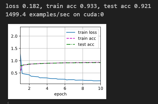
最后看一下测试效果：

#VGG-11计算量太大，这里构建了一个四分之一尺寸的网络来训练,计算量为1/16,但依然很大

ratio = 4
small_conv_arch = [(pair[0], pair[1] // ratio) for pair in conv_arch]
net = vgg(small_conv_arch)

lr, num_epochs, batch_size = 0.05, 10, 128
train_iter, test_iter = d2l.load_data_fashion_mnist(batch_size, resize = 224)
d2l.train_ch6(net, train_iter, test_iter, num_epochs, lr, d2l.try_gpu())

批量归一化

批量归一化（BN）是深度学习中的一种数据标准化技术。在神经网络的每一层之间，它会对数据进行重新调整，强制让它们的分布回到均值为 0、方差为 1 的状态（在训练时计算当前的均值方差，测试时会使用预训练好的均值方差）。

优势如下：

• ​训练提速（Speed Up） ：它能解决“梯度消失”问题，允许我们使用更大的学习率，让模型收敛速度提升数倍。
• ​降低敏感度（Robustness） ：它让模型对权重初始化不那么挑剔。即使初始化做得一般，模型也能稳定训练。
• ​正则化效果（Regularization） ：BN 在训练时引入了微小的噪声，这能起到类似 Dropout 的作用，防止模型过拟合，提高泛化能力。

3. 它的标准位置

在现代卷积神经网络中，它就像“三明治”的中间层：

卷积层 (Conv) $\rightarrow$ 批量归一化 (BN) $\rightarrow$ 激活函数 (ReLU)

在 pytorch 中实现也很简单：

nn.BatchNorm1d(x) # x 为通道数

ResNet

ResNet 的想法

我们希望向模型添加更多的层以增加深度，期望降低任务误差。从 LeNet 到 GoogLeNet，深度逐渐增加的模型也获得了更好的性能。但是深度增加，模型的效果一定更好吗，并不见得是这样的。

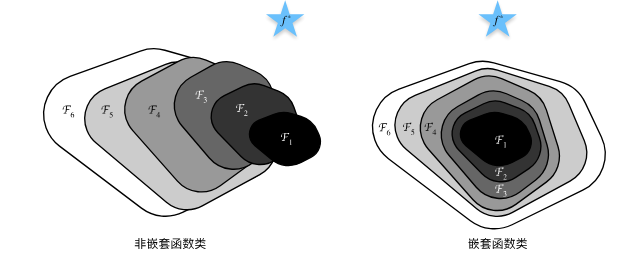
于是，我们意识到：添加层以加深神经网络的目的，是为了扩展原有模型的表达能力，使其能够表示更复杂的输入输出映射。在最差的情况下，新添加的层没有学到任何有用的特征，新模型也能完整地退化为原有模型，不改变已有的输入输出映射。​​

这一恒等映射的引入，限制了深度网络扩展时的性能下界、避免了不必要的复杂度的产生、提供了进一步优化的可能性。这正是何凯明等人于 2016 年提出的​残差网络 (Residual Network, ResNet) 的核心思想：让新添加的层学习来自输入的残差，而不直接拟合输出，实现更稳定、高效的网络。该网络模型在 2015 年 ImageNet 图像识别挑战赛中夺魁，深刻影响了后来的深度神经网络设计。

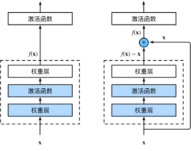
如图所示，假设我们的原始输入为 x，而希望学出的理想映射为 f(x)。 左图虚线框中的部分需要直接拟合出该映射，而右图虚线框中的部分则需要拟合出残差映射。 以本节开头提到的恒等映射作为我们希望学出的理想映射，我们只需将右图虚线框内上方的加权运算（如仿射）的权重和偏置参数设成 0，那么即为恒等映射。 实际中，当理想映射极接近于恒等映射时，残差映射也易于捕捉恒等映射的细微波动。 右图是 ResNet 的基础架构–残差块（residual block）。 在残差块中，输入可通过跨层数据线路更快地向前传播。

• ​通堆叠（左图） ：当你往网络里多加一层时，新得到的函数集合不一定包含原来的函数集合。也就是说，加了新层后，网络可能反而找不到之前那个较浅状态下的最优解了。
• ​理想状态​：我们希望加了新层后，网络至少能表现得和没加之前一样好。如果新层能学到“​恒等映射”（即输入是什么，输出就是什么），那么性能就不会下降。

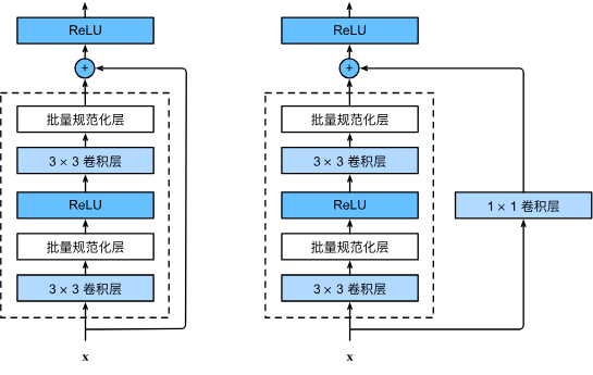
ResNet 沿用了 VGG 完整的 33 卷积层设计。 残差块里首先有 2 个有相同输出通道数的 33 卷积层。 每个卷积层后接一个批量规范化层和 ReLU 激活函数。 然后我们通过跨层数据通路，跳过这 2 个卷积运算，将输入直接加在最后的 ReLU 激活函数前。 这样的设计要求 2 个卷积层的输出与输入形状一样，从而使它们可以相加。 如果想改变通道数，就需要引入一个额外的 1*1 卷积层来将输入变换成需要的形状后再做相加运算。 残差块的实现如下：

import torch
from torch import nn
from torch.nn import functional as F
from d2l import torch as d2l


class Residual(nn.Module):  #@save
    def __init__(self, input_channels, num_channels,
                 use_1x1conv=False, strides=1):
        super().__init__()
        self.conv1 = nn.Conv2d(input_channels, num_channels,
                               kernel_size=3, padding=1, stride=strides)
        self.conv2 = nn.Conv2d(num_channels, num_channels,
                               kernel_size=3, padding=1)
        if use_1x1conv:
            self.conv3 = nn.Conv2d(input_channels, num_channels,
                                   kernel_size=1, stride=strides)
        else:
            self.conv3 = None
        self.bn1 = nn.BatchNorm2d(num_channels)
        self.bn2 = nn.BatchNorm2d(num_channels)

    def forward(self, X):
        Y = F.relu(self.bn1(self.conv1(X)))
        Y = self.bn2(self.conv2(Y))
        if self.conv3:
            X = self.conv3(X)
        Y += X
        return F.relu(Y)

在代码中还需要考虑维度对齐的问题，因为经过一个残差块后 x 和 f(x)的形状可能不一样，所以需要一个 1*1 卷积核来维度对齐。如下图所示：

模型的实现如下：

def resnet_block(input_channels, num_channels, num_residuals,
                 first_block=False):
    blk = []
    for i in range(num_residuals):
        if i == 0 and not first_block:
            blk.append(Residual(input_channels, num_channels,
                                use_1x1conv=True, strides=2))
        else:
            blk.append(Residual(num_channels, num_channels))
    return blk

b1 = nn.Sequential(nn.Conv2d(1, 64, kernel_size=7, stride=2, padding=3),
                   nn.BatchNorm2d(64), nn.ReLU(),
                   nn.MaxPool2d(kernel_size=3, stride=2, padding=1))
b2 = nn.Sequential(*resnet_block(64, 64, 2, first_block=True))
b3 = nn.Sequential(*resnet_block(64, 128, 2))
b4 = nn.Sequential(*resnet_block(128, 256, 2))
b5 = nn.Sequential(*resnet_block(256, 512, 2))
net = nn.Sequential(b1, b2, b3, b4, b5,
                    nn.AdaptiveAvgPool2d((1,1)),
                    nn.Flatten(), nn.Linear(512, 10))

X = torch.rand(size=(1, 1, 224, 224))
for layer in net:
    X = layer(X)
    print(layer.__class__.__name__,'output shape:\t', X.shape)

Sequential output shape:	 torch.Size([1, 64, 56, 56])
Sequential output shape:	 torch.Size([1, 64, 56, 56])
Sequential output shape:	 torch.Size([1, 128, 28, 28])
Sequential output shape:	 torch.Size([1, 256, 14, 14])
Sequential output shape:	 torch.Size([1, 512, 7, 7])
AdaptiveAvgPool2d output shape:	 torch.Size([1, 512, 1, 1])
Flatten output shape:	 torch.Size([1, 512])
Linear output shape:	 torch.Size([1, 10])

ResNet 的梯度计算

残差块的前向传播逻辑可以简化为：

\[y = x + \mathcal{F}(x)\]

其中 x 是输入，F(x) 是残差路径（包含卷积、BN 和激活函数）的输出。

当进行反向传播计算损失函数 L 对输入 x 的梯度时，根据链式法则：

\[\frac{\partial L}{\partial x} = \frac{\partial L}{\partial y} \cdot \frac{\partial y}{\partial x}\]

由于 y = x + F(x)，我们对 x 求导得到：

\[\frac{\partial y}{\partial x} = \frac{\partial (x + \mathcal{F}(x))}{\partial x} = 1 + \frac{\partial \mathcal{F}(x)}{\partial x}\]

因此，梯度的传递公式变为：

\[\frac{\partial L}{\partial x} = \frac{\partial L}{\partial y} \cdot \left( 1 + \frac{\partial \mathcal{F}(x)}{\partial x} \right) = \frac{\partial L}{\partial y} + \frac{\partial L}{\partial y} \cdot \frac{\partial \mathcal{F}(x)}{\partial x}\]

这个公式揭示了两个极其重要的特性：

• ​梯度“高速公路” ：式子中的第一个项 $\frac{\partial L}{\partial y}$ 代表梯度可以毫无损耗地通过快速通道直接传回到前一层。

• ​打破连乘效应：

  • 在普通网络中，梯度是多层权重矩阵的​连乘。如果权重很小，梯度会呈指数级衰减。
  • 在 ResNet 中，梯度变成了加法形式。即便中间权重层的梯度 $\frac{\partial \mathcal{F}(x)}{\partial x}$ 变得非常小，由于那个“1”的存在，总梯度依然能够保持在 $\frac{\partial L}{\partial y}$ 左右，保证了底层参数能接收到有效的更新信号。

如果我们把网络看作是多个残差块的堆叠，从深层 L 到浅层 l 的梯度流向可以表示为：

\[\frac{\partial L}{\partial x_l} = \frac{\partial L}{\partial x_L} \cdot \left( 1 + \sum_{i=l}^{L-1} \frac{\partial \mathcal{F}(x_i)}{\partial x_i} \right)\]

• ​求和而非求积：这种性质使得梯度即便经过几十个残差块，也不会轻易塌缩为 0。
• ​参数更新稳定：这让每一层都能得到合理的更新，从而让深层网络也能获得极高的准确率。

残差的梯度计算通过将“梯度连乘”改为“梯度直通”，为神经网络修建了一条直达底层的“梯度高速公路”，使得万亿参数、极深层次的现代 AI 模型（如 BERT 和 GPT）的训练成为可能。